The Context Engineering Stack
Part 2 / Context EngineeringThe four layers
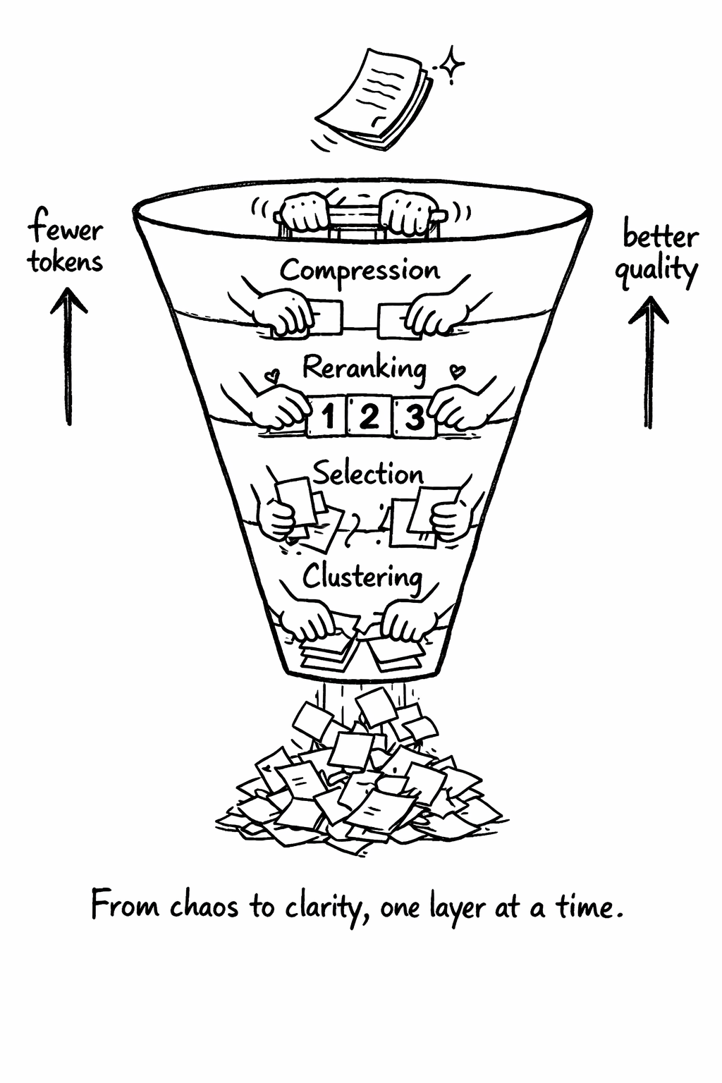
Context engineering operates in four layers, each addressing a different problem. These layers form a pipeline: raw retrieved content enters at the bottom and curated, compressed context exits at the top. Each layer reduces token count while preserving - or improving - information quality. Understanding these layers is essential because most teams only implement retrieval (getting chunks from a vector database) and skip the post-retrieval processing that determines whether those chunks actually help the model.
Layer 1: Clustering
When you retrieve 10 chunks from a vector database, they often contain the same information expressed differently. Your documentation says the same thing as your code comments. Your FAQ overlaps with your support tickets. Your API reference restates what’s already in the tutorial. Without clustering, you send all of these to the model, wasting tokens on redundancy and confusing the model with multiple phrasings of the same fact.
Clustering groups semantically similar chunks together using their embedding vectors. Agglomerative clustering works well for this because it doesn’t require you to specify the number of clusters upfront - it adapts to your data by starting with each chunk as its own cluster and progressively merging the most similar pairs until a distance threshold is reached.
The distance threshold is the key parameter. Set it too low and you get too many clusters (not enough deduplication). Set it too high and you merge chunks that are related but distinct. A cosine distance threshold of 0.15-0.25 works well for most documentation and code contexts. You should tune this on your own data by inspecting the clusters and verifying that merged chunks genuinely express the same information.
When five chunks all say “the API rate limit is 100 requests per minute,” they should be recognized as expressing the same fact. When two chunks discuss rate limiting but one covers the REST API and the other covers the WebSocket API, they should remain separate. Getting this distinction right is what makes clustering useful rather than destructive.
Layer 2: Selection
After clustering, you need to pick the best representative from each cluster. This is where domain knowledge matters - the “best” representative depends on what you’re trying to accomplish.
For coding tasks, the best representative is usually the most specific one - the code file itself rather than the documentation about the code, the test file rather than the test plan, the error message rather than the error handling guide. Agents work better with concrete examples than with abstract descriptions.
For research tasks, the best representative is usually the most authoritative one - the primary source rather than a summary, the official documentation rather than a blog post, the peer-reviewed paper rather than the preprint.
For customer-facing tasks, the best representative is usually the most recent one - the latest policy rather than the historical policy, the current pricing rather than the old pricing, the updated FAQ rather than the original FAQ.
“Best” depends on your use case:
| Selection Strategy | When to Use |
|---|---|
| Most detailed | Technical documentation, API references |
| Most recent | Rapidly changing codebases, changelogs |
| Most authoritative | Security policies, compliance docs |
| Shortest | Token-constrained scenarios |
The key insight: you don’t need all five versions of the same fact. You need one good one.
Layer 3: Reranking
After selection, rerank the remaining chunks to balance relevance and diversity. The initial retrieval from your vector database uses bi-encoder models - they embed the query and the documents independently, then compare the embeddings. This is fast but imprecise. Two documents can have similar embeddings without being relevant to the same query.
Maximal Marginal Relevance (MMR) addresses this by balancing relevance (how similar is this chunk to the query?) with diversity (how different is this chunk from chunks already selected?). The λ parameter controls the trade-off: - λ = 1.0: Pure relevance (may include redundant chunks)
- λ = 0.0: Pure diversity (may include irrelevant chunks) - λ = 0.7: Good default for most use cases
The reranking step typically changes the order of 30-50% of the documents. The documents that move up are the ones that are specifically relevant to the query and different from other selected chunks. The documents that move down are the ones that are either not specifically relevant or too similar to other selected chunks. This reordering directly improves the model’s output because the context contains diverse, relevant information rather than redundant variations of the same information.
This prevents the failure mode where your top 10 results are all slight variations of the same information.
Layer 4: Compression
The final layer removes redundancy without losing signal. The critical decision here is deterministic versus non-deterministic compression.
| Approach | Latency | Cost | Deterministic | Debuggable |
|---|---|---|---|---|
| LLM-based summarization | ~500ms | $0.01/call | No | No |
| Algorithmic deduplication | ~12ms | $0.0001/call | Yes | Yes |
LLM-based summarization uses a language model to condense the selected chunks into a shorter summary. It produces readable output but introduces non-determinism - the same input can produce different summaries on different runs. This makes debugging nearly impossible. When an agent produces bad output, you need to reproduce the exact context it received. If the compression layer is non-deterministic, you can’t.
Algorithmic deduplication uses deterministic techniques - sentence-level deduplication, overlap removal, structural compression - to reduce token count without changing the content. It’s faster, cheaper, and reproducible. The output isn’t as polished as an LLM summary, but for agent consumption (not human reading), polish doesn’t matter. What matters is that the information is accurate, complete, and reproducible.
For production systems, determinism is a requirement. You need to reproduce problems, audit decisions, and debug issues. You can’t do that if your preprocessing layer gives different answers on different days. Use algorithmic compression in production and reserve LLM-based summarization for offline analysis where reproducibility isn’t critical.
Distill: A reference implementation
Distill is an open-source context engineering tool that implements all four layers - clustering, selection, reranking, and compression - in a single pipeline. It was built to solve a specific problem: monorepo context is too large and too redundant for direct inclusion in agent context windows.
The design philosophy behind Distill is determinism over quality. Every operation in the pipeline is deterministic - the same input always produces the same output. This means you can reproduce problems, audit decisions, and debug issues. It also means you can cache aggressively - if the input hasn’t changed, the output won’t change either.
Distill processes context in four steps. First, it embeds all chunks using a sentence transformer model (all-MiniLM-L6-v2 by default, configurable). Second, it clusters similar chunks using agglomerative clustering with a configurable distance threshold. Third, it selects the best representative from each cluster based on a configurable strategy (most detailed, most recent, most authoritative, or shortest). Fourth, it removes redundancy within the selected chunks using algorithmic deduplication - sentence-level overlap detection and removal.
The result is a compressed context that preserves the information content of the original while using 60-80% fewer tokens. For a typical monorepo with 45K tokens of relevant context, Distill reduces it to 12K tokens with less than 2% information loss (measured by downstream task accuracy).
Results from production deployments:
| Metric | Before Distill | After Distill | Improvement |
|---|---|---|---|
| Context tokens | 45K | 12K | 73% reduction |
| Redundant chunks | 30-40% | <2% | ~95% reduction |
| Output consistency | 62% | 89% | +27 percentage points |
| Cost per request | $0.135 | $0.036 | 73% reduction |
| Latency | 8.2s | 2.1s | 74% reduction |
Meta-MCP: Compressing tool definitions
A pattern from the Japanese developer community (documented on Zenn.dev) addresses a specific context engineering problem: tool definition bloat.
When you connect 60+ MCP tools, the tool descriptions alone consume 15-20K tokens. Each tool needs a name, a description, a parameter schema with types and descriptions, and often usage examples. Multiply that by 60 tools and you’ve consumed a significant portion of your context window before the agent has even started working.
The meta-MCP pattern compresses these into 2 meta-tools: a discovery tool that returns a list of available tools with brief descriptions, and a load tool that loads the full definition of a specific tool when the agent needs it. Instead of sending all 60 tool definitions in every request, the agent first asks “what tools are available?” (consuming ~2K tokens for the list), then loads only the tools it needs for the current task (consuming ~500 tokens per tool).
The result is dramatic: tool definition overhead drops from 15-20K tokens to 2-4K tokens - an 80-88% reduction. For a 200K context window, this frees up 15K tokens for actual content. Over a 20-turn session, the cumulative savings are even larger because the reduced tool definitions are included in every turn.
The meta-MCP pattern has a trade-off: the agent needs an extra tool call to discover and load tools, which adds latency (typically 200-500ms) and a small amount of cost. For most use cases, this trade-off is overwhelmingly positive - the token savings far outweigh the extra tool call cost.
Context engineering for different agent types
Different types of agents need different context engineering strategies.
Coding agents need codebase context - file contents, directory structure, git history, test results, and AGENTS.md instructions. The key challenge is selecting which files to include. A naive approach (include all files in the repository) quickly exceeds the context window. A better approach uses the agent’s task description to identify relevant files - if the task is “fix the login bug,” include the login-related files, their tests, and their dependencies. Codebase knowledge graphs (Chapter 6) make this selection more accurate.
Research agents need document context - papers, articles, web pages, and internal documentation. The key challenge is deduplication - the same information often appears in multiple sources. The context engineering stack (clustering, selection, reranking, compression) is essential for research agents.
Operations agents need system context - logs, metrics, configuration files, and deployment state. The key challenge is recency
- operations context changes rapidly, and stale context leads to incorrect actions. Operations agents should always fetch fresh context rather than relying on cached data.
Customer-facing agents need conversation context - the user’s history, preferences, and current intent. The key challenge is privacy - customer data must be handled according to your data protection policies, and PII must be redacted before it enters the model’s context.
Related Concepts: Context Window (4.1), Token Budget (4.3) Related Workflows: Implementing Meta-MCP for Token Reduction (Chapter 23)